

In other documents we have show you how to use the Visual Crossing Weather Data Services capability to do Query API loading of weather data directly into Excel.
There are three primary Excel use cases for Weather Data.
1) Load a fixed query set of data into a table and reference that table for further analysis.
Loading Weather Data into Excel via Web Query URL
2) A variation on the fixed query load is the 15-day forecast query which is dynamically always showing the next 15 days from “today”. So while the URL Query doesn’t change, the users will add a refresh option either manually or on load of the spreadsheet.
How to automaticall refresh weather data in Microsoft Excel
3) Dynamically pass in data to replace parameters in the API Query string based upon Excel data. Users will want to pass in locations, lists of locations, dates and other parameters. In this document we will focus on this option.
The Initial Query String
First let’s repeat what we have done in previous queries and visit the Visual Crossing Query Builder page and build a simple one-location query for Forecast data and load it into Excel. Follow along with steps from link found in number 1 above which uses the following page:
https://dev.visualcrossing.com/weather-query-builder/
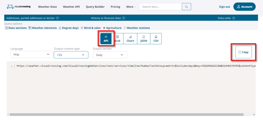
Once you have a successful forecast data query, switch to the API tab to see our query string. Make sure the language drop down is set to ‘Http’ and the Output content type one to ‘CSV’. Click on the ‘Copy’ button to put the string in our system copy/paste buffer:
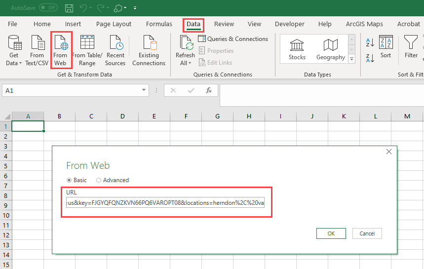
Next we load it into Excel by visiting the “Data” tab, selecting the “From Web” option and pasting in our URL String copied from the Visual Crossing Weather Data Query Builder above.
Click ‘OK’ and ask to Load the data which will give us the following working query:
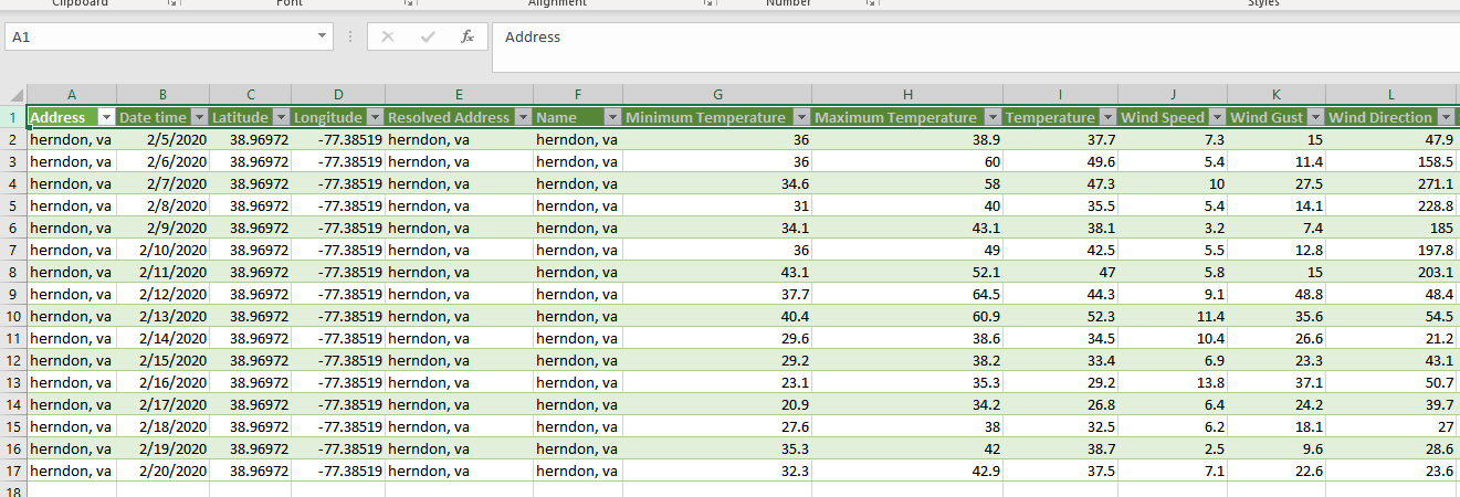
This is the step where the other document ends but here we will begin to use parameters to customize this query.
Preparing Data for the Query
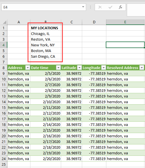
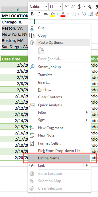
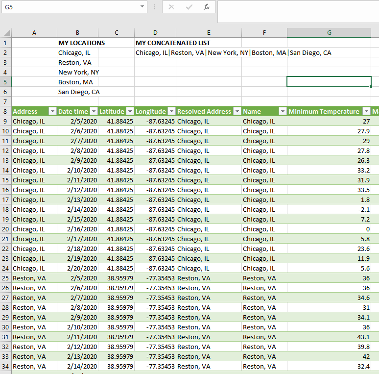
The first step is to insert some blank rows at the top of the page and enter in a list of 5 locations. This is just an area of cells with no real definition for now but will serve as our data entry area so that our users can simply update this list to get weather for these locations. To build this area simply type in the cells as seen below. Please note that we put a header “MY LOCATIONS” but this is not necessary and should not be in the data table we define. It is just for clarity.
Select the list of Cities (without the header) and create a defined table name for this area. The easiest is to Right-click on the locations selection and use the “Define Name” option. We will name our table “RAWLIST” for now.
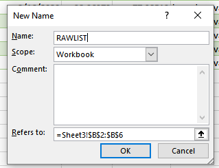
This range is now defined and can be accessed from anywhere simply by referencing RAWLIST. However, if you prefer you can also use your own literal range definitions of cells such as “b2:b6”.
Now it is our job to make sure this list can be insert into the query so that we can retrieve multiple locations dynamically. The first step is to concatenate the list into a string that can be inserted into the URL. We want our list of city cells to be in a single string such as “Chicago, IL|Reston, VA|New York, NY”. Please note that the query has to have a list that is delimited by the pipe “|” symbol.
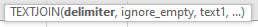
To do this we will use the TEXTJOIN function in Excel. (Please note that there many ways to create this same list in Excel so feel free to use your favorite technique) Click into a new cell and insert the following function.
For our example it looks like the following:
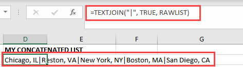
The first Parameter is the pipe symbol in quotes to define our delimiter, we put in “TRUE” as the second paramter to ignore any empty cells and we reference our table range called “RAWLIST” as the final parameter which is the list of locations.
Please note in the image above that we have a nicely joined single string ready to insert into the query. We will again right-click on our cell and give it a range name using the “Define Name” feature. We will call this range “WxLOCATIONS”.
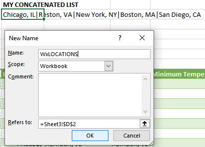
NOTE: Previously we used the named range feature for ease of use, but for the next exercise it is required that our concatenated list has a name. We will refer to this name in the query steps.
Inserting Parameters into the Query
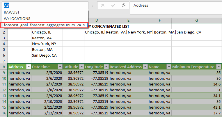
Lets starting by selecting our query that we made in step one, the easiest way to do this is to select it from the list of ranges as seen below or use the “Queries & Connections” window to select it.
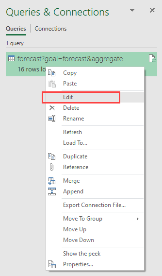
On the right hand side of the sheet you should now see the “Queries & Connections” window. Select our query and right-click to choose to ‘Edit’ this query.
The query editor will open up as seen below and we have chosen the ‘Advanced Editor’ view:
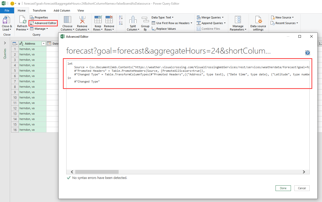
Once opened you can see the text of query. If you look closely you will see the string that we copied from the Visual Crossing Weather Query Builder in the ‘Source’ definition. But notice that our string is only part of the query which also defines columns, types and many other pieces of metadata. We must be careful to only edit the portion we pasted in.
The first thing we need to do is to define a variable that will contain our concatenated list. To do this enter the following text above the ‘Source’ entry:
WxLoc=Excel.CurrentWorkbook(){[Name="WxLOCATIONS"]}[Content]{0}[Column1],
This new line is telling the query to define “WxLoc” as the contents of the WxLOCATIONS range from the current workbook. It is asking for the first row (row zero) of the default ‘Column1’ name. We only have one row and one column for our concatenated string anyway. Please make certain to have the comma at the end of the text to indicate the end of your variable Definition for “WxLoc”. Here is what your query should look like:
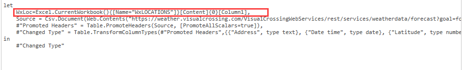
The last edit is to our original query string. Find the following text in the ‘Source’ definition:

The string says “Herndon, VA” with some escape characters, this is becauseour original query was a hardcoded query to one location at Herndon, VA. Now we need to make the locations definition dynamic. Simply replace the text after the “locations=” and before the closing parenthesis with the following:
"&WxLoc&" "
and will now look like:
locations="&WxLoc&" ")
We are basically saying that the first part of our query string + ‘OUR LOCATIONS LIST’ + last part of our query string is our new string. Effectively we are concatenating a variable into the query string by cutting out the hardcoded “Herndon, VA” string and inserting our dynamic concatenated string.
Once this is in place, the query will now dynamically grab our locations list and use it in the query to the Visual Crossing Weather Engine whenever the query is refreshed.
We can now click ‘Done’ on this query editor and the system will validate your string changes. If you get an error just double check your work and naming. Usually a misplaced quote or comma is the culprit. If successful you may see a warning from the system that looks like this:
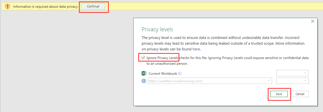
This warning is Excel telling you that it is sending your data (list of locations) to a remote server and it needs your permission to do this. You can set the permission levels that serve your scenario best. For this exercise we will choose to Ignore the Privacy Levels, Save it and click ‘Continue’ on the warning bar.
Now we can see the results of our new query in the query preview window:
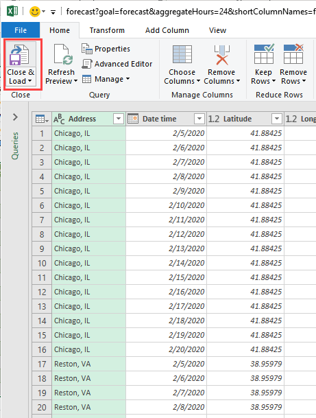
We can now verify that it is returning weather data for our list of cities. Just click ‘Close and Load’ to finish the query. Now we are back in our workbook and we can see the results of our work.
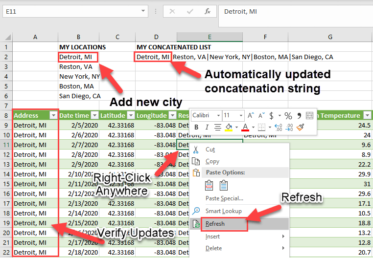
Test and Add Features
To test our work further you can update the list and then click ‘Refresh’ on the query and it will update the data live.
Please remember to set your refresh policy. Above we simply right clicked on the query results and chose ‘Refresh’. Our document here describes the common ways to refresh the query data automatically:
How to automatically refresh Weather Data in Microsoft Excel
However, this scenario may call for more user interaction such as putting in a button or dynamically detecting changes in your table range. All of which can be enabled easily using VBA objects. We found the simplest variation was to use the ‘Developer’ tab on the Ribbon Bar (may need to be added to the ribbon) and add a button then record a refresh Macro for the button to activate. There are many other enhancements here such as adding dynamic checklists of locations, hiding the concatenation string and much more, but we will leave that to the Excel expert in you to explore.