

.We use a lot of sources for our weather data. One of the richest sources of historical weather data is the Integrated Surface Database (ISD) from NOAA. The amount of data available is impressive. Hourly or sub-hourly weather records for 1000s of weather stations that are, in some cases, over 100 years old. However obtaining and manipulating the data so that it fits your needs can be a daunting task. In this article we describe some of the lessons we’ve learned along the way and some of the processes that we use to make the data as useful as possible.
Visual Crossing Weather Data now includes real time weather history data from the MADIS weather observations database.
Our Weather Data Services page offers historical weather data download, query and weather API building features that make it easy to get the weather data you need.
What is the Integrated Surface Database?
The Integrated Surface Database (often abbreviated to ISD) is a large collection of hourly and sub-hourly weather observations collected from around the world. The result is a large database of weather information in a consistent, text-based format.
Choosing the right dataset
There are multiple ISD datasets available within the ISD product set. There are three main datasets of raw data available on the ISD – full file download (consisting of the full hourly/subhourly data), ISD Lite and the Daily Summaries. Depending on your use case, you should choose the simplest set that satisfies your requirements.
Daily Summaries
The daily summaries dataset provides the values of the summary weather observations for a full day. This gives the minimum/maximum temperatures for the day, total precipitation (rainfall, snow etc) and other observation parameters. If you are looking for data at the day level only and don’t require hourly level data, this is the best dataset to work with. However one thing to note is that you are subject to the day aggregation algorithm provided by the data. This may introduce problems with rainfall being recorded on the incorrect day as we will discuss below.
Hourly Global
The full ISD dataset includes Global hourly and synoptic observations compiled from numerous sources. Within this data you will find that there are weather observations that span sub-hourly, hourly, 3 hourly, 6 hourly, daily summaries and monthly summaries. This is an incredibly rich dataset but does take additional work to extract the data and ensure it is consistent. We are going to focus on this dataset in this article because we find there are some data features only available when using the full dataset.
Hourly Global ISD Lite
In many cases the ISD Lite dataset may serve your requirements better than the full Hourly Global dataset. This dataset has been processed so that it is hourly records with no subhourly or other time periods. We have used this for various projects but it does have limitations regarding the precipitation records. ISD Lite FTP Access.
Reading the data for a location
ISD datasets are recorded by weather station. The process for finding the ISD records for a particular location is therefore to find the closest station (or group of stations) near the location of interest. After finding the stations, you can load the data files for the date range that you are concerned with.
Finding the right weather station
The Integrated Surface Database includes a full list of weather stations in the isd-history.txt file. This includes the station description, latitude, longitude and weather station IDs along with some useful information regarding the weather station.
If I know the name of a local weather station, I can search the list. For example, here is Washington Dulles International Airport:
724030 93738 WASHINGTON DULLES INTERNATION US VA KIAD +38.935 -077.447 +0088.4 19730101 20190516
If you don’t know the name of the local weather station, it would be necessary to search the list by latitude and longitude, or by country or US State abbrevation.
It is important to remember that this is the full list of weather stations that feature in over 100 years of data collection. Most of those weather stations do not have records covering the full time period. To verify that a station does have data, another index file is available: isd-inventory.txt.
We can use this file to identify what years and months have useful data. From the station list, we can see the that Dulles Airport is USAF ID 724030. We can use this ID in the inventory dataset to identify the data:
724030 93738 1973 812 706 893 799 775 780 794 823 767 813 745 867
...
724030 93738 2018 1035 1028 1044 989 1155 1058 1071 1046 1171 1045 1015 1077
724030 93738 2019 1096 982 1019 977 597 0 0 0 0 0 0 0
Multiple rows are returned for each station with each row corresponding to a year of data that may be available. Here we can see that the record began in 1973 and continues to the present day. The twelve numbers in each row represent the number of observations available for each month of the year. Given we hope these records are hourly, we can quickly identify whether the dataset inventory suggests a good quality dataset. With 24 hours per day, we would expect from 672 records for a 28 day month up to 744 in a 31 day month. As the inventory records higher numbers, this indicates that we can expect to see other rows such as sub-hourly and summary records and that the records for this weather station look good from 1973 onwards.
Armed with the station IDs, we can now download the actual data. There are two ways to do this – for a single station or in bulk for all stations in a year.
The global hourly access folder (https://www.ncei.noaa.gov/data/global-hourly/access/) provides the starting web accessible location for individual records. You can then browse for the year and station. For example here is the URL for our Washington Dulles example above for 2019 data:
https://www.ncei.noaa.gov/data/global-hourly/access/2019/72403093738.csv
Note that the file name 72403093738.csv is created by joining both the USAF and WBAN Ids together.
If you are looking for data for many stations, then you can also download all the available station data for a single year at https://www.ncei.noaa.gov/data/global-hourly/archive/csv/. For recent years this is a very large amount of data even when compressed. 2018 data is 4.5Gb compressed (nearly 47Gb uncompressed)!
Data format documentation
Now that we have data for our station, we can start using it. Detailed documentation on the ISD format can be found at isd-format-document.pdf and it’s useful to have this available as a quick reference. A supplemental document https://www.ncei.noaa.gov/data/global-hourly/doc/CSV_HELP.pdf provides help specifically for the CSV (command separated values) file format that we are using.
The data is a CSV text format so can be opened up in a text editor or any tool that supports reading CSV files. In this document I am going to use Microsoft Excel for screenshots of the file to help make the discussion easier to follow.
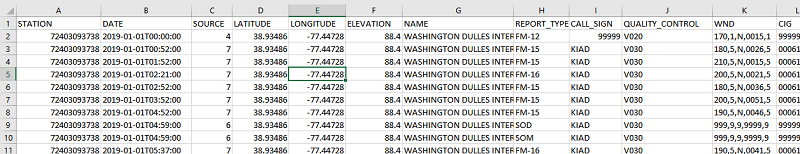
When we open the file of 2019 data for Washington Dulles Airport, we see that each row represents a single observation. Each observation includes a set of standard values such as the Station ID, the date and time of the observation, the source, latitude and longitude. Note that the latitude and longitude values are often of higher precision than the values given in the above isd-history.txt station list.
Identifying hourly records
Before we can extract weather observations from the data, we must first identify the records we are interested in. In our case we are primarily interested in the hourly level data. What is the temperature each hour? How much did it rain in the past hour? What is the wind speed?
To do this, we want only the hourly data. As you can see from the date times on the above screenshot, it is not obviously clear what observation represents the hourly observation. Looking down the observations, we see times at 52 minutes past the hour and also others at 11, 32 47 minutes. We need to identify the observations that represent the current hourly data.
To help identify the records of interest, we can first use the REPORT_TYPE field to eliminate some records. The documentation describes many types. Some of them we can eliminate immediately:
-
- SOD – Summary of Day. A summary of the weather observations for the previous 24 hours
-
- SOM – Summary of Month. A summary of the weather observations for the previous month
-
- PCP15 – US 15-minute precipitation network report
-
- PCP60 – US 60-minute precipitation network report
After eliminating records with types that we cannot use, we still need to eliminate records where there are multiple records for every hour. But which record should we choose to represent the hourly observation? Fortunately we have help from NOAA because we can take advantage of the logic used by the Lite data format discussed above.
Duplicate Removal
In many cases, there can be more than one element at the same observation time or within the capture window. In these situations, a single element is chosen from the list of duplicates according to a ranking schema. The ranking schema assigns a score to each element according to these criteria: Difference between actual observation time (minute) and the top of the hour.
Observations that are closer to the top of the hour are favored.Ranking of the data quality flag from the ISD observation. Generally, observations with a higher data quality flag (i.e. passed all quality control checks) are favored over observations with a lower data quality flag (i.e. suspect).Ranking of the data source flag from the ISD observation. Observations that come from a merger of datasets are favored over elements that have not been merged (i.e. datsav3/td3280/td3240 merged elements are favored over just datsav3).Ranking of the report type code from the ISD observation.
Observations that are formed from merger of multiple report types are favored over observations that are not (i.e. merger of Synoptic/Metar is favored over just Synoptic).A score is assigned to each of these tests, favoring the order listed above. The observation with this highest score is chosen to be the hourly value. In case of a tie score, the element that was encountered first in the original ISD file is chosen.
Using this we have now reduced our records to the records that are hourly based. Typically those records will be on a regular time each hour (normally in the 10 minutes before the hour). If you see records that have a consistent minute value then that is likely the best hourly observation record to use. In the case of our Washington Dulles Airport dataset, the hourly records are nearly always record at 52 minutes past the hour.
It is worth repeating at this stage that the Lite version of the data does a lot of this work for you if you aren’t affected by some of the limitations we will discuss below.
Time zone and aggregated values
We have now identified the hourly records and we are nearly ready to start looking at the observed values. However before we do that we need to consider the times of the observations. All of the times in the datasets are recorded at UTC time (also known as GMT/Greenwich Mean time). Therefore you need to transform the time to local times in most cases. This is particularly important if you are intending to compare the hourly data to another dataset. At Washington Dulles Airport, which is four or five hours behind UTC, comparing temperatures at midday vs seven o’clock in the morning would cause a signficant error!
Another more complex impact of the time difference is that some summary data can occur in the incorrect day. Consider precipitation data that is always recorded based on the total precipitation over a preceding time period. If you use a 24 hour total you might use the following:

As we will see in a later discussion, this record is indicating a 24 hour period total precipitation of 13.5mm (roughly 0.5″). The date of this observation is 1/1/2019 however it is a UTC time that looks back 24 hours. The rainfall actually occurred the day before – on 31st December 2018. Many web sites that use daily aggregated data will actually report precipitation on the incorrect date because they report the UTC date of the 24 hour summary observation and don’t take into account the backwards looking nature of this observation. Unfortunately precipitation records are made further complex by inconsistent reporting etc. We will therefore return to this discussion in the section dedicated to precipitation.
Reading observations
We are finally ready to read some weather data from the dataset. We can start with some simple values:
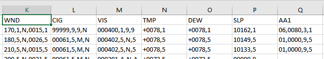
As you can see, most observation values are not simple numbers but rather a sequence of number fields separated by a comma. Each observation value normally includes at least the actual measured value and a quality indicator.
So for example ,’TMP’ refers to the temperature observation +0078,1. In this case, “+0078” indicates the temperature in Celsius. The temperature value is scaled by 10 to avoid requiring decimal places in the database. Therefore the temperature is 7.8C or 46.0F. The second part indicates the quality (1 = Passed all quality control checks). The ISD documentation includes a reference of quality codes you can expect to see. Finally if we saw a value of +9999 then we would know the value is missing.
The value of ‘WND’ is 170,1,N,0015,1. WND represents wind measurements of the form direction,direction quality,observation type, speed, speed quality. Again the speed is multipled by 10 to avoid using decimal points in the file format. Therefore this record indicates that the wind direction was 170 degrees with a speed of 1.5 meters per second (approximately 3.4mph or 5.4 kph).
The format of having a scaled value (often by 10), with a quality indicator and using +9999 for missing is a very common constuct within the file. The ISD documentation describes exactly what values can be expected.
Handling precipitation records
Some records are more involved than the temperature and wind speed observations. Precipitation records in particular warrant special consideration. There are a number of factors that make precipitation more complex:
-
- Precipitation is often recorded for multiple hour periods. The periods can vary from one hour to 24 hours and often varies for the same weather station
-
- Hourly precipitation records are often not available except in recent years
-
- In many cases, multiple hour precipitation totals do not equal the sum of the hourly totals
Let’s look at some precipitation data from our Washington Dulles Airport location:
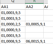
For these records, we can see that there are two columns for precipitation observations (there can be up to three). The precipitation record is of the form period,accumulation,condition,quality. For the two values we therefore have:
-
- 01,0003,9,5 – a one hour period with 0.3mm of rainfall.
-
- 03,0005,9,1 – a three hour period with 0.5mm of rainfall.
In this dataset, we have both hourly data, in addition to three, six and 24 hour period summaries. We can use the summary data to double check the hourly data (even here you can observe a slight difference in total). In the cause of a station that does not report hourly data, you can choose to split a multiple hour period value amongst hours if you are looking to report hourly data (with obvious approximation, particularly if you are splitting a 24 hour period).
As we have shown, determining low level precipitation values can take a reasonable amount of data cleansing. However for many applications being able to compare exactly when it rained compared to particular events (eg store footfall, national park visitor counts etc.) is important, so it is worth extra effort. Once you know what hours have experienced rain, you can also measure the precipitation coverage. Precipitation Coverage can demonstrate data trends based on how long it rains for, not just how much it rains.
Missing and erroneous data
In many cases you will find that stations do not report data for particular time period. For example, we have even found instances of all the stations near Chicago going offline for many days! When processing ISD data, effective measures should be taken to mitigate this. The best approach is to compare to surrounding stations. Comparing to surrounding stations will also help identify erroneous values in addition to missing values. For smaller size projects, performing this step manually is perfectly reasonable. For larger projects other techniques, such as interpolation, should be considered.
Station interpolation and dataset gridding
In some of our larger projects we need a fast historical data look up for many locations concurrently. To do this we create a grid of pre-processed historical data so that we can easily query the historical data records. This has a number of advantages:
-
- We pre-process the data cleansing so we can make the cleansing more rigourous even if it takes additional processing power
-
- We have the ability to interpolate values from multiple stations
-
- We significantly reduce the amount of data that is stored by eliminating repeated data (such as the id, name and latitude and longitude of the weather station we see recorded on every observation line in the raw files).
For each cell we typically consider the surrounding weather stations within 50-100km. We then take the results from each station and eliminate any missing observations. After cleaning using the above rules, we then aggregate values weighting closer stations more than farther stations. We do this at the individual observation level so that short term missing data is accommodated. This approach gives us the best results for possible missing data, station inconsistencies etc.
Applications of the data
The data available through the NOAA Integrated Surface Database (ISD) are extremely rich. The data contains hour-resolution historical weather observations for many worldwide locations and for many years in history (and it’s always improving!)
To try looking up some historical weather data right now, check out our Weather Data page.