

Does your business depend upon knowing when freezing temperatures may occur? Shipping temperatures sensitive items, water pipes/pumps, pouring concrete or outdoor employee safety are just a few areas where businesses can benefit by knowing exactly when a freezing temperature is predicted.
Typically, systems like this can be a very expensive IT undertaking but in this post we will show you how to get started for budget-friendly sum. We will start with a scenario where you will need to know everyday, possible forecasts that include freezing temperatures anywhere in the US. This type of scenario would help anyone who ships products scan the entire US in a simple to read single Excel spreadsheet. Lets get started…
To build this Excel Workbook you will need an Excel version later than 2016 and you will need a Visual Crossing Account. If you haven’t already signed up for an account please do so here:
Please note that even a free account should work fine for this effort but you cannot create a scheduled dataset that updates automatically and you have to make sure your query stays under the 1000/day limit.
If you are not able to follow along and build your own workbook, at the bottom of this post you can find the download to our final product. The final workbook comes with a fixed file of data loaded on GitHub called SampleFreezeData.csv . You will replace that link with your live link copied from the ‘My Datasets’ section of Query Builder to analyze your own data.
Step 1 – Build a Weather Dataset
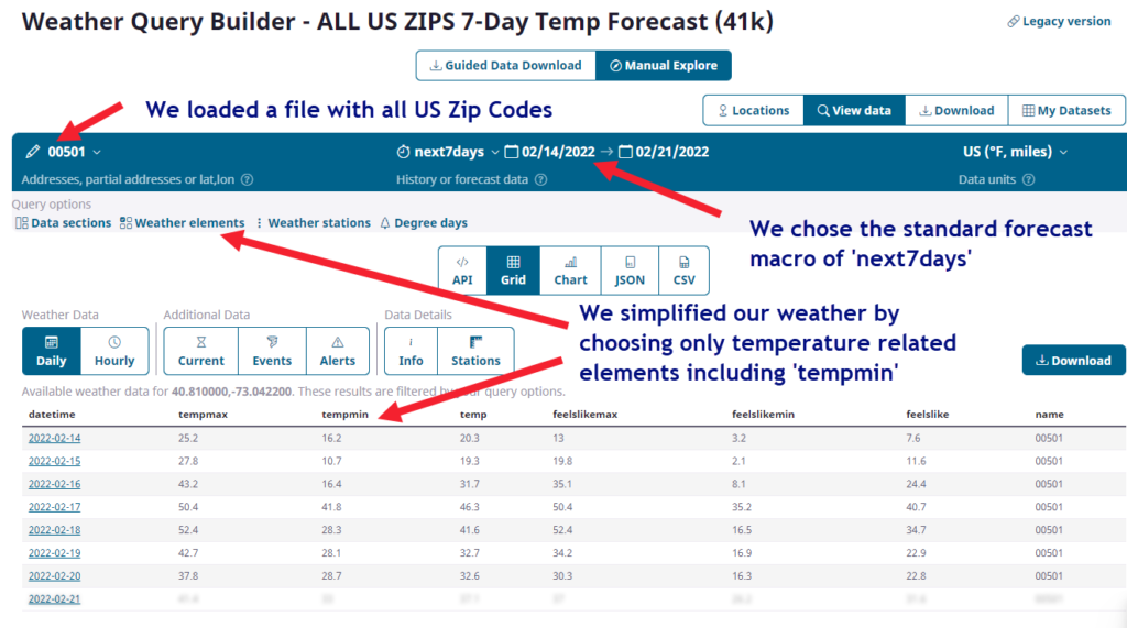
The first step is to set up and build the forecast dataset that you will need. In our example we are going to take on a larger project and use one of the standard datasets that are available to our Corporate Licensed Customers as a standard bulk dataset. It is a forecast weather query for all us zip codes. This way, regardless of how many areas we will ship to, we can cover the whole US and simply avoid shipments to these areas. For your use case you may wish to start smaller and build a query with a handful of locations. If you are new to building saved and scheduled datasets, please follow this tutorial:
In the above blog it also has links to another tutorial and saving your dataset as a schedule. In a final solution you may wish to set up your own but it is not required for this exercise. You can simply run a dataset and be able to access the link to it from ‘My Datasets’ section of the Query Builder.
Here is a quick view of the Zip Code dataset that we outlined for this exercise:
Step 2 – Download & Prepare Weather Workbook
You may or may not be aware of our Weather Workbook downloads. These are sample Excel workbooks that take on the job of pulling weather data directly into our workbooks. The latest version of this workbook uses datasets to pull data directly into Excel via the Power Query capabilities of later Excel versions. In this overview of Weather Workbook for Datasets it includes a link to download a copy to your local environment. Here is where you can find it:
To create our Freezing Temperature Workbook, we will build upon this workbook. The download link to base workbook is here for your ease of access. Please click on it and download a copy if you want to follow along building your own. Please note that we are providing links to our finished product in this post.
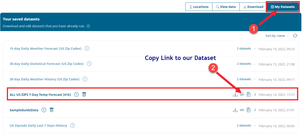
From reading the ‘how to build a dataset…’ blog we know how to copy a dataset link from ‘My Datasets’. We will go there now and retrieve our dataset link that we will use for this workbook.
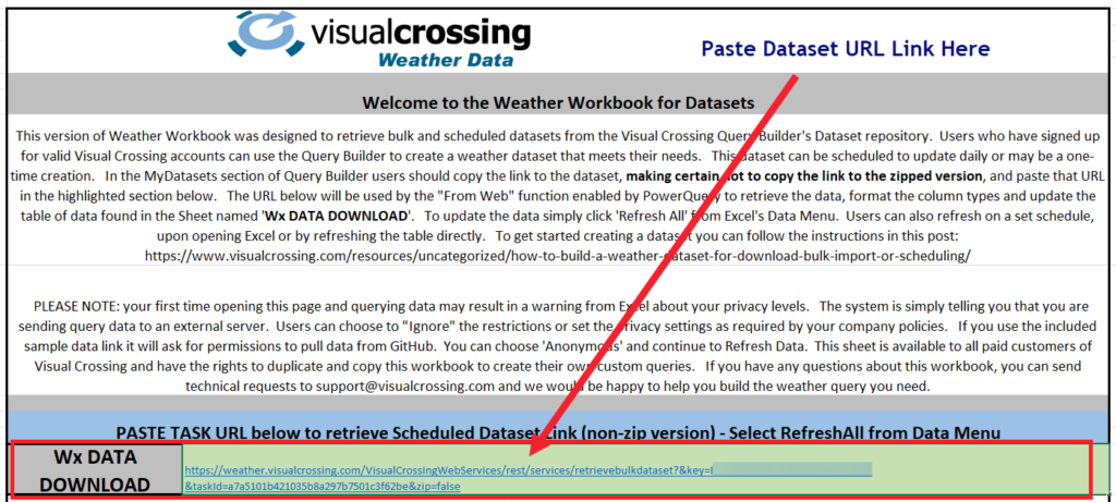
The string URL link is now in our copy-paste buffer. Now open Weather Workbook and paste in our link into the green highlighted area replacing the link that is currently there.
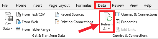
We can now navigate to the Data menu in Excel and choose ‘Refresh All’.
By doing this we are asking Weather Workbook to use the URL link to download the whole dataset into our workbook. This may take a few minutes depending upon the size of your dataset. Our data is 41,000 rows x 7 days forecast or ~290,000 rows of data.
Once your dataset is downloaded please check the dataset in the ‘Wx Data Download’ sheet of the workbook:

This sheet contains all of the results for the query in raw format. In our next steps we are going to copy the existing query.
NOTE: At this point it is also a good idea to save your workbook just in case you want to refer back to it or unroll changes as we progress.
Step 3 – Duplicate Our Query into a Pivot Table
Now that we have a fully working query, we are going to make a copy of it but we are going to begin to build our calendar of locations and dates by emptying our data into a Pivot Table to make it easier to read and format. This will make us more efficient in identifying parts of the US that will freeze in the coming week.
As seen below, navigate to the Data menu in Excel and open the ‘Queries & Connections’ editor which will open in the right sidebar. Then right click on our query and choose ‘Duplicate’.
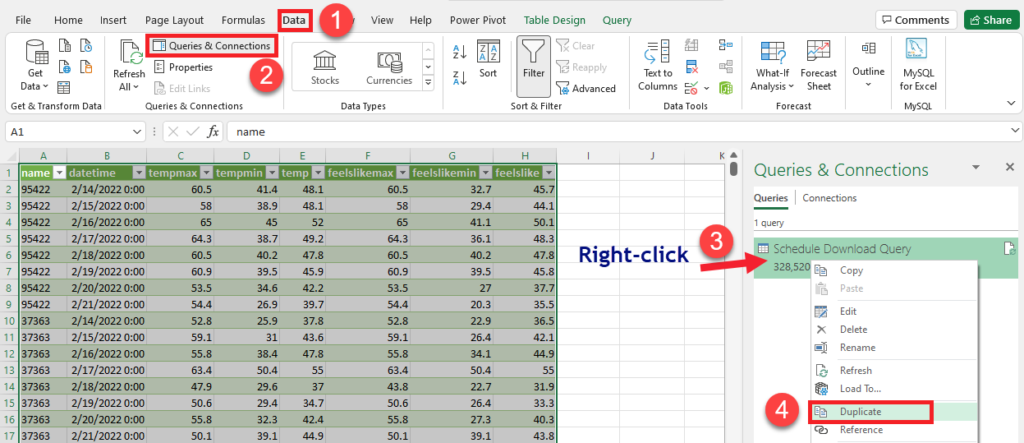
This will create a second query in our list and open the advanced editor automatically for us to edit, save and load our new query as we see below.
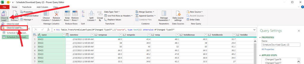
All we need to do is pull down the ‘Close & Load’ menu and choose ‘Close & Load To’. This option will offer to us a few options of where to put the data in Excel.
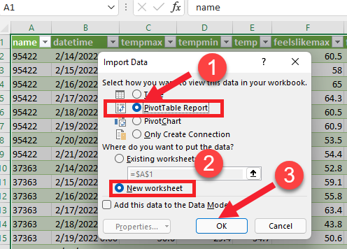
For this excercise we are going to use the ‘PivotTable Report’ in a new worksheet and click ‘OK’ to finish.
We now have our data loaded into the pivot table structure but we haven’t selected data yet. Use the field list at the right to drag fields over to create calendar view of our data where our dates are in the columns. If the field window is not open for you simply right-click on the Table Area and ‘Show Field List’.
Step 4 – Assign Data and Format the Pivot Table
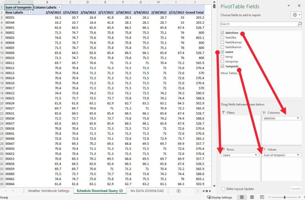
When we drag the data to the appropriate areas we will see our data. We put ‘name’ in the rows (this is just our location name which is our zip codes), we put ‘datetime’ in the columns and finally we put tempmin into the ‘Values’ area. NOTE: If we add a second value to this area a special ‘Values’ placeholder will appear and should be placed on the rows.
One key item we need to do is to select the ‘Sum of tempmin’ field in the ‘Values’ area to define the aggregation of our min temperature value and name it.
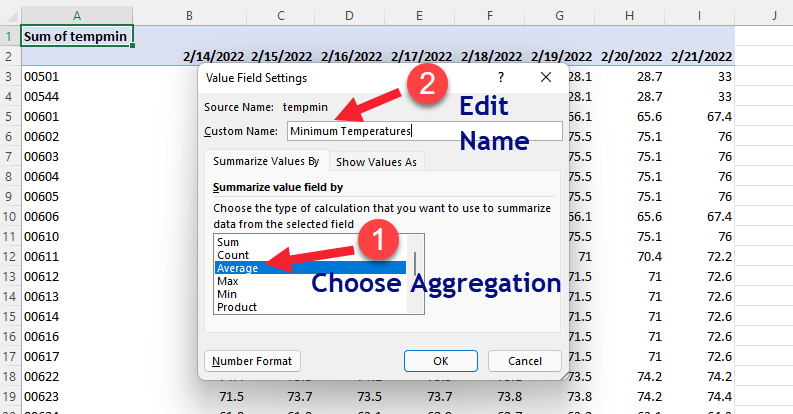
Here we will set any total aggregations to be an average of all min values, Sum and Count do not make sense, but you may choose to have a minimum of our values to see the coldest possible. Then we will rename our value to a more user friendly name such as ‘Min Temperature’.
The final step is to make our Pivot Table look more readable. To do this right-click on the Pivot Table and open the Options editor.
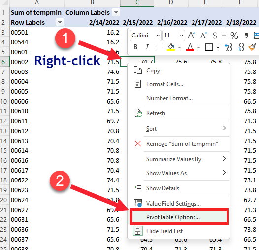
We will leave this section open to you but we have chosen to turn off all totals, outlines and labels and keep our table simple and clean for easy viewing.
We have now loaded our data into pivot table. The only problem is that it is difficult to identify the freezing temp with 40,000 rows of data. We need a better user interface so we will begin by adding a Conditional Format to our Pivot Table. To do this, we need to give our users the ability to set the minimum value they are searching for. We don’t want to hardcode a value as different industries and companies require different freeze settings.
Step 5 – Add a Temperature Alert Rule
Navigate back to the ‘Weather Workbook Settings’ and we will add a section for users to add a value.
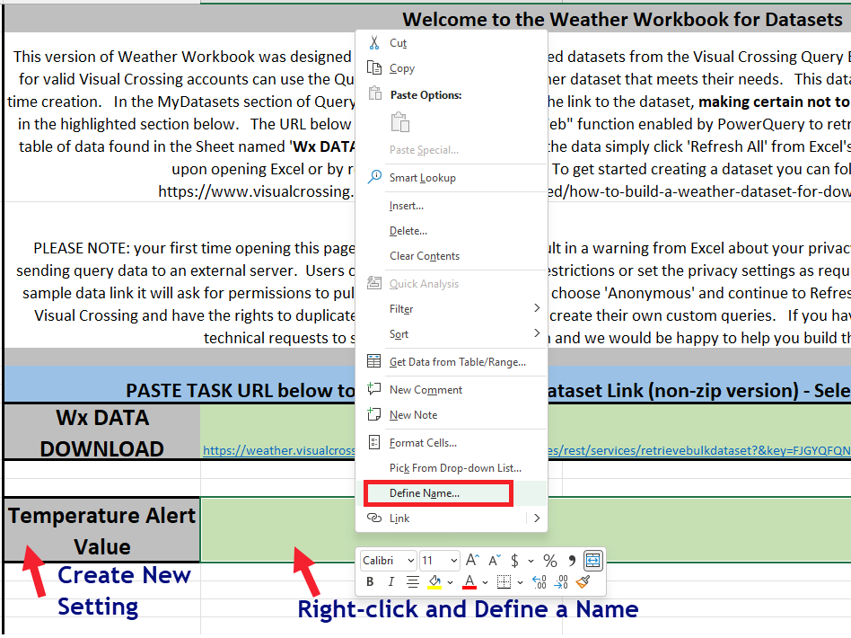
Start by creating a pair of cells similar to our ‘Wx DATA DOWNLOAD’ entry area. One column is just a friendly name and the green section will be our actual data section. Once you create the green cell, right-click and select ‘Define Name…’. This will allow us to name this area and read that value from anywhere in our workbook.
We will enter the name ‘TEMPALERT’. Once you do this and click ok, you can see in the workbook that whenever you select the cell, the upper left hand list of named areas will show our name.
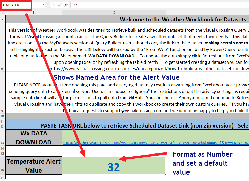
We can finish by putting in a value, making sure it is formatted as a number. Also make sure that you only have one cell and it isn’t merged. We will set ’32’ as our default but you can change this anytime.
Now we can navigate back to our copied query where we created the pivot table. Now we can set our freeze threshold rule.
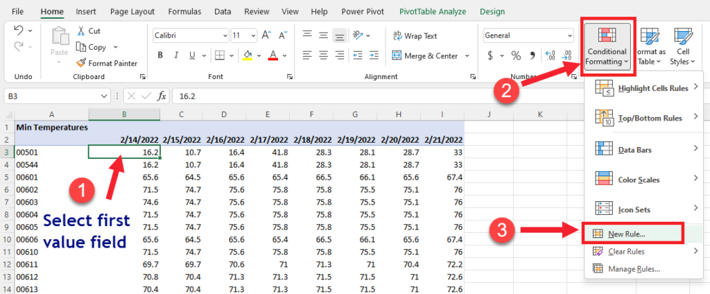
Start by selecting our first value cell for minimum temperature. Next we will open the ‘Conditional Formatting’ menu on the ribbon bar and select ‘New Rule…’.
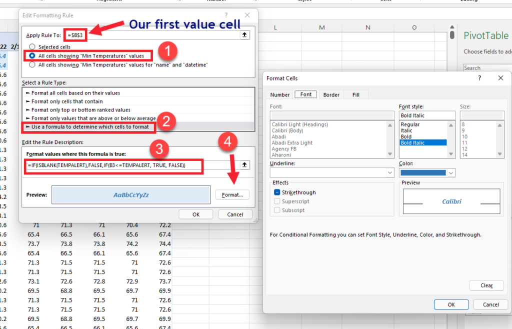
When the editor opens we will first note that it believes that we are applying the rule to the cell we selected. First we will tell the rule to apply to all cells for our ‘MinTemperatures’ field not just the one cell. Next we will define the rule by selecting the option to use a formula. Next we can enter in our formula… Note that here we can define a simple formula that simple says ‘=B3<TEMPALERT’ and this will do the correct thing most of the time. However, it doesn’t account for null values in the setting or in the data. So we will use the following formula:
=IF(ISBLANK(TEMPALERT),FALSE,IF(B3<=TEMPALERT, TRUE, FALSE))It is a bit complex but just note that the rule will color the cell in our data when values are less than or equal to our value set in the ‘TEMPALERT’ area.
Finally, you can format your alert cells by clicking on the ‘Format…’ button and coloring the text and/or background. We chose dark blue font on light blue background in bold.
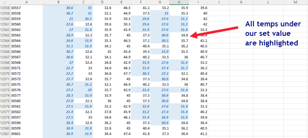
click ‘OK’ and finish the rule and you will see that it is automatically applied and is now highlighting the days and zip codes that have freezing temperatures in our 7-day forecast.
You are welcome to play with the ‘TEMPALERT’ value and set it to values that are meaningful to your business. The Pivot Table will automatically apply any changes you make, there is no need to refresh data.
Step 6 – Conclusions
There are many customizations that can be done to this workbook to tailor it to your needs but what we have given you here is a budget-friendly way to retrieve freeze data and analyze a week of forecast for thousands of locations. If your license allows, you can simply set up your dataset as a schedule and use the ‘Refresh All’ option under the ‘Data’ menu to update your Excel data to grab the latest dataset from the server.
Remember that you can download and use the workbook we created and simply swap out your dataset link and start analyzing today.
NOTE: The workbook comes with a fixed file of data loaded on GitHub called SampleFreezeData. You will replace this link with your live link copied from the ‘My Datasets’ section of Query Builder to analyze your own data.