
This tutorial will guide you through the process of joining an existing Excel sheet to both historical and forecast weather data using Visual Crossing Weather Add-in for Microsoft Excel. For sample data we will use a sheet containing several store locations on the US East Coast. First-time users are encouraged to walk through the process using this sample data so that you understand the steps required to join and use the tool. Once you are familiar with the process using this sample data, you should be able to easy apply the same concepts to your own data. First, if you have not already done so, please open the Visual Crossing Weather Tutorial workbook supplied with this tutorial.
To follow along with this tutorial, please download the example Workbook attached to the bottom of this article.
Step 1: Install the Visual Crossing Weather for Microsoft Excel add-in from the Microsoft App Source store.
To install the Visual Crossing control, please visit the Microsoft Excel Weather Data home page and sign up for a trial or purchase of the Visual Crossing Weather add-in. Once you do so, you should be able to see an icon like the one below under My Add-ins when running Microsoft Excel.
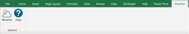
Clicking and installing the add-in will add a Weather entry to your Excel menu bar. Clicking on the Weather menu option will show the options below.
Step 2: Logging into Visual Crossing Weather
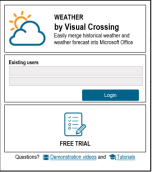
You will now need to log into Visual Crossing Weather. The first step is to click on the Weather icon shown above. The Weather panel will open on the right-hand side of your Excel sheet. You will then see a login box as shown below. If you already have a Visual Crossing account, you can enter the appropriate login and password. If not, click on the Free Trial button and walk through the process of signing up for your free trial account.
Weather History
Step 3: Select the source historical data
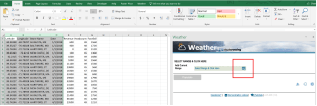
We will begin by joining our business data dates with historical weather data. To do so, ensure that the workbook is set to the Store History tab and select the first four columns (Latitude, Longitude, Store Name, and Date). (Note that we could have used addresses here instead of latitude and longitude values. However, since our data already has latitude and longitudes for the store locations, we will use them directly.)
Please note that trial users are limited to 100 rows. If you submit more than 100 rows in your range, the populate action will trigger an error and inform you to reduce your range size.
Once you have selected those columns, press the Select Range button in the Weather tab.
Step 4: Join your existing sheet with historical weather data
When you click the Select Range button as described above, you will see that Visual Crossing Weather automatically populates options based on the data that you have provided. In this case, it has found latitude and longitude values, and a date column. The date column signals that you wish to join historical weather data to match the existing sheet dates.
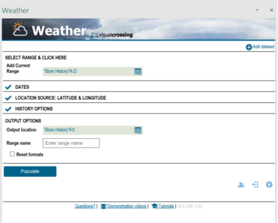
Note that you can easily select the individual sections (such as Date, Location Source, etc.) in the Weather panel and make manual adjustments if the appropriate columns were not guessed correctly. For our example data, however, the columns will be guessed properly.
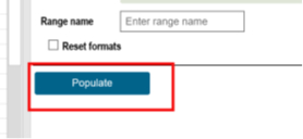
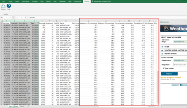
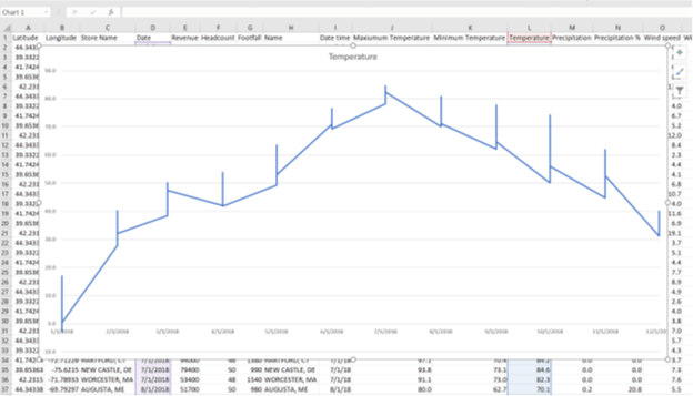
Now that the data has been selected and options populated, you can click the Populate button at the bottom of the Weather panel. This will cause several new columns to be added to the right of the existing sheet data. These columns contain the weather at the specified locations (given by the latitude/longitude) and on the specified dates. You will see variables such as Temperature, Precipitation, and Wind speed. (Note that you can use the options on the Weather panel to change the output location if you wish.)
Your sheet should now look like this.
Step 5: Analyze the weather history at the locations
You can now use the power of Excel’s rich analysis functionality to analyze the weather events at the given locations. For example, below is a simple graph that shows how the temperature changes at the locations throughout the year. You can obtain it simply by selecting the date and temperature column and inserting a line graph. The analysis possibilities are limitless.
Weather Forecast
Step 6: Select the forecast locations
Next switch to the Stores tab in the Excel workbook. There you will find several store locations that match the locations we used for the history section above. Select the three columns on this sheet (Latitude, Longitude, and Store Name) and then click the Range Selection button.
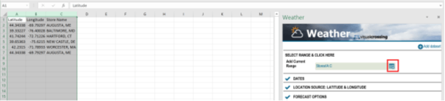
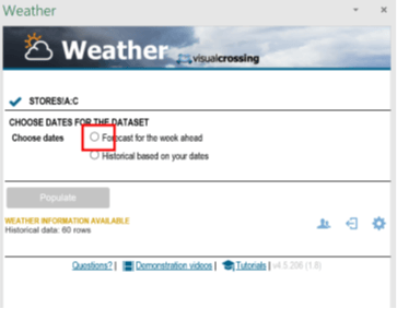
As before, this will cause Visual Crossing Weather to analyze the data and select the appropriate options. However, in this case, there is no date on our data, so Visual Crossing does not know if you want to do an historical analysis or a forecast. Thus, the Weather panel prompts us to choose. Simply select the radio button for “Forecast for the week ahead” since we are interested in forecast data analysis now.
Visual Crossing Weather will now finish analyzing your input data and populate the other options. (Note that you can easily change these if you wish, but for this tutorial we will stay with the defaults.)
Step 7: Populate the forecast data for the selected locations
You can now press the Populate button at the bottom of the Weather panel
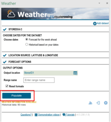
This will cause Visual Crossing Weather to populate the forecast data on the sheet to the right of the location data. (Note as before that you can easily change this output location via the panel settings.) This new data shows the forecast details for each location over the next week. Your sheet should now look approximately like the sheet below.
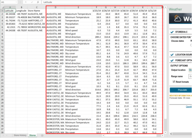
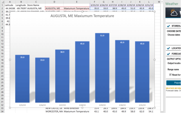
Step 5: Analyze the weather forecast
As with the historical weather data, this new forecast data is now available for you to analyze in Excel. For example, you can select the first two rows of forecast data and make a graph of the temperature in Augusta during the coming week.